February 27, 2021
My daughter shared a lovely problem she had encountered in her calculus class: I was inspired to make a Desmos animation: FTC (Evaluation part)
"If others would but reflect on mathematical truths as deeply and as continuously as I have, they would make my discoveries." - Carl Friedrich Gauss
February 27, 2021
My daughter shared a lovely problem she had encountered in her calculus class: I was inspired to make a Desmos animation: FTC (Evaluation part)
August 4, 2019
Here’s what my colleagues Travis Ortogero, Robert Machemer, and I have come up with as an alternative to expensive, heavy textbooks for our precalculus classes. Some sections are more fleshed out than others. We make incremental improvements as we have the time and energy.
September 6, 2018
The homework assignment I gave my AP Calculus class on the first day of school this year was inspired by Michael Pershan’s well-worth-a-read post I don’t focus my classroom on solving problems. (This was his contribution to Sam Shah‘s fabulous Virtual Conference on Mathematical Flavors). In developing Read more…
February 20, 2017
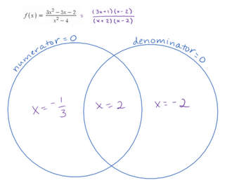
I’ve been teaching for 27 years. This morning during a discussion of rational functions in a precalculus class, I had one of those why-didn’t-I-think-of this-years-ago moments, when I found myself drawing a Venn diagram on the board in response to massive confusion about holes. My hypothesis about Read more…
January 30, 2017
Inspired by Annie Perkins and her post “For Those Hesitant to Protest” and prodded by a friend to share the following more widely, I offer here the following passage which was my contribution our family’s Christmas letter to family and friends this year. While I do enjoy Read more…

July 24, 2016
Exponential growth is a topic that deserves especially thoughtful treatment as part of a high school education because a person who has thought deeply about this ubiquitous phenomenon pays attention to and conceptualizes certain critical issues in, for example, science, economics, and social science, in a fundamentally different way than one who Read more…